Motivation for using smaller number format?
- reduce memory footprint
- reduce memory bandwidth pressure
- enables packing more math units into same silicon area
- consume less energy
Linear Operations Can Cheaply Deal with Scales
Let:
- $x = (x_i | 1 \leq i \leq k)$ be a vector of reals.
- $x^q$ be the integer-quantized version of $x$.
- $x’ = (x_i^q * dscale_x | 1 \leq i \leq k)$ be the approximation of $x$ after dequantization.
- Define $y$ and $y’$ similarly.
Then,
$$ z’ = \sum_i x’_i * y’_i = dscale_x * dscale_y \sum_i x_i^q * y_i^q $$
Most of the math is cheap, only the dequantization at the end is expensive.
what is the effect of quantization on the performance of the model?
- reduce the range, scaling factor clips the value to the range [min, max]
- reduce the precision, rounding the value to the nearest integer
Scaling Factor Granularity:
- per-block quantization: $x^q = (x_{i,j,k}^q | 1 \leq i \leq k, 1 \leq j \leq m, 1 \leq k \leq n)$
- per-tensor quantization: $x^q = (x_i^q | 1 \leq i \leq k)$
- per-channel quantization: $x^q = (x_{i,j}^q | 1 \leq i \leq k, 1 \leq j \leq m)$
- per-layer quantization: $x^q = (x_{i,j,k}^q | 1 \leq i \leq k, 1 \leq j \leq m, 1 \leq k \leq n)$
Quantization Design Space:
How to choose quantization scheme? (TBD)
How to compensatre for for quantization error?
Quantization Techniques
K-Mean Quantization
Quantization by clustering: Use k-means to find the best set of centroids for the given tensor. As a result, a tensor is compressed into low-bits index and a cookbook.
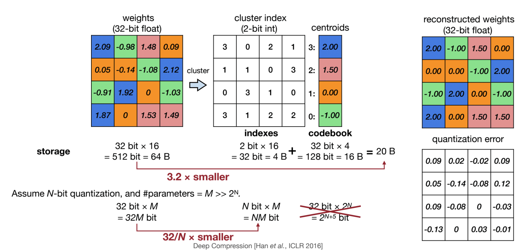
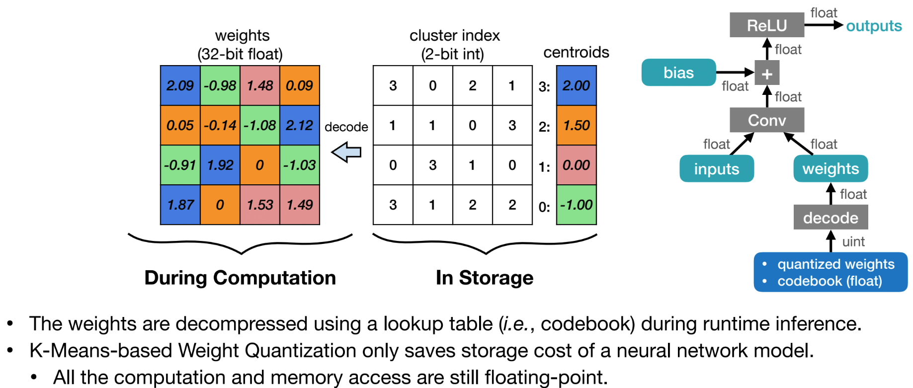
Weights are decoded by “cookbook” table lookup. Reduce memory footprint and memory bandwidth pressure, all computation is still in full FP.
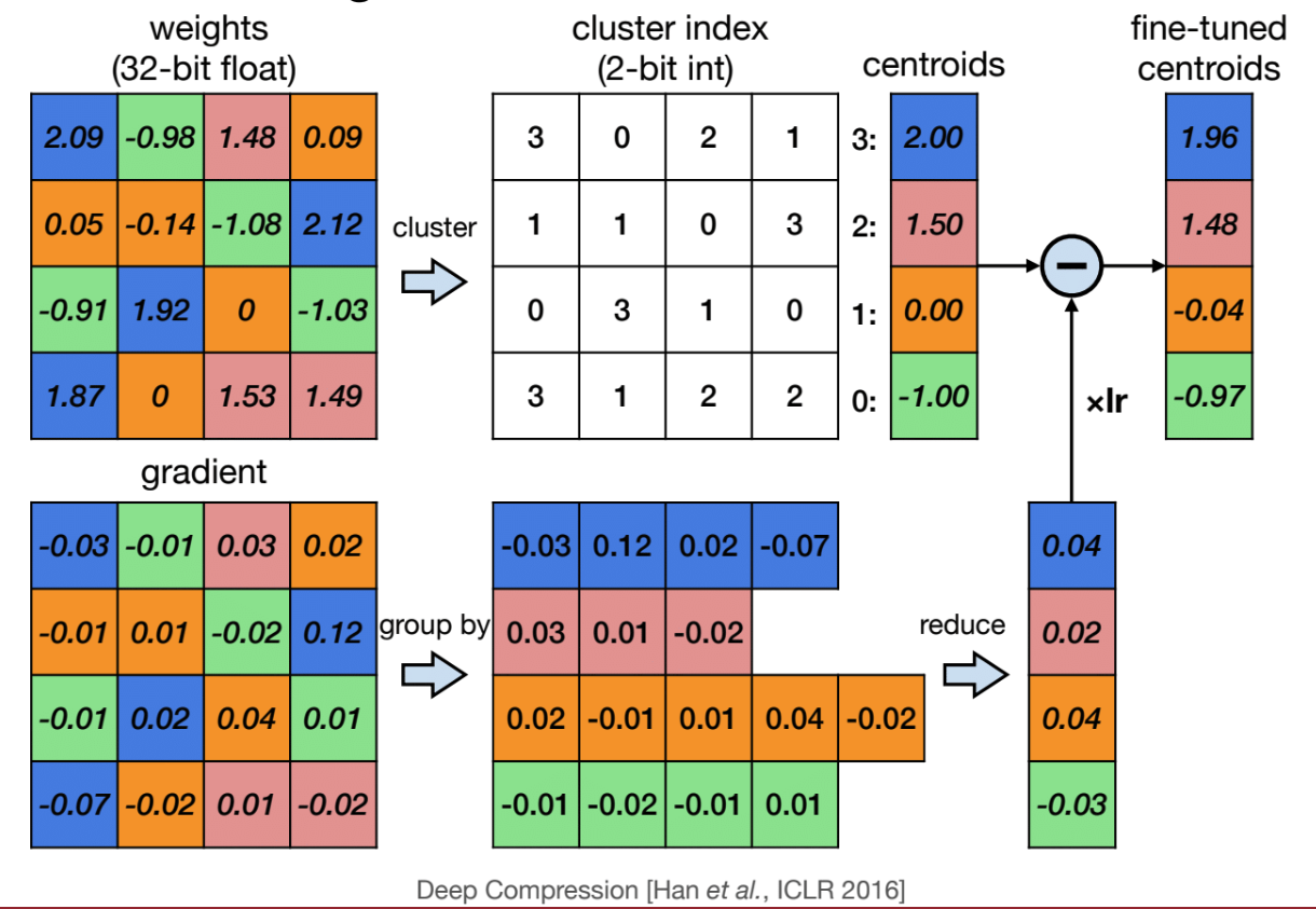
To recover model accuracy, weights in K-mean quantization are optimized by gradient descent to update the centroids.
Linear Quantization
Affine mapping between integer and real numbers:
$$ A \approx (A^q - z ) * s $$
- $A \in \mathbf{R}^{m \times n}$
- $A^q \in \mathbf{Z}^{m \times n}$ where $Z$ is N-bit integer
- $z \in \mathbf{Z}$ is the zero-point
- $s \in \mathbf{R}$ is the scaling factor
How to calcuate $z$ and $s$?
$r_{min}$ and $r_{max}$ are the minimum and maximum values of the real numbers in the matrix $A$. $q_{min}$ and $q_{max}$ are the minimum and maximum values of the N-bit integer numbers.
$$ r_{max} = s(q_{max} - z) \ r_{min} = s(q_{min} - z) $$
then we have:
$$ s = \frac{r_{max} - r_{min}}{q_{max} - q_{min}}
z = q_{max} - \frac{r_{max}}{s} \
$$
$s$ is the ratio between dynamic range of the real numbers to the N-bit integer numbers.
Given $s$, we can calculate $z$ as follows:
$$ z = q_{max} - \frac{r_{max}}{s} $$
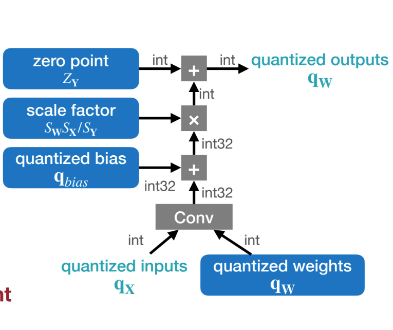
Matrix Multiplication with Linear Quantization
$$ \begin{aligned} Y &= WX \ &\Rightarrow s_y(Y^q - z_y) = s_w(W^q - z_w) * s_x(X^q - z_x) \ &\Rightarrow q_y = \frac{s_w s_x}{s_y} (W^q - z_w)(X^q - z_x) + z_y \ &\Rightarrow q_y = \frac{s_w s_x}{s_y} (W^q X^q - z_w X^q - z_x W^q + z_w z_x) + z_y \end{aligned} $$
Empirically, weights distribution is symmetric around 0, so $z_w$ is set to 0. Then we simplify the equation as follows:
$$ q_y = \frac{s_w s_x}{s_y} (W^q X^q - z_x W^q) + z_y \ $$
At inference time, $W^q$ and $z_x$ are constant (pre-determined), thus $z_x W^q$ can be pre-computed. The bulk of runtime computation is the integer matrix multiplication of $W^qX^q$.
Similarly, for matrix product with bias, we have: $$ \begin{aligned} Y &= WX + b \ &\Rightarrow s_y(Y^q - z_y) = s_w(W^q - z_w) * s_x(X^q - z_x) + s_b(\mathbf{b}^q - z_b) \ &\Rightarrow q_y = \frac{s_w s_x}{s_y} (W^q X^q - z_x W^q) + \frac{s_b}{s_y} (\mathbf{b}^q - z_b) + z_y \ \end{aligned} $$
Since weight and bias follows the same distribution, we can force $s_b = s_ws_x$, and $z_b = 0$, then we have:
$$ q_y = \frac{s_w s_x}{s_y} (W^q X^q + B^q) + z_y \ $$
where $B^q = -z_x W^q + \mathbf{b}^q$ is pre-computed and does not change at runtime.
Linear layer with activation function, i.e. ReLU, can be quantized using the same technique as matrix multiplication.
$$ \begin{aligned} q_y &= \frac{s_w s_x}{s_y} (Linear(X^q, W^q) + B^q) + z_y \ &\Rightarrow q_y = \frac{s_w s_x}{s_y} (ReLU(W^q X^q) + B^q) + z_y \ \end{aligned} $$
ReLU is essentially a clipping operation: $ReLU(x) = max(0, x)$. With proper quantization parameters (output activation $s_y$ and zero-point $z_y$), this clipping happens “for free” during the de-quantization process. We can simplify the equation as follows:
$$ q_y = \frac{s_w s_x}{s_y} (W^q X^q + B^q) + z_y \ $$
Convolution with Linear Quantization
Convolution is linear operation, so it can be quantized using the same technique as matrix multiplication.
$$ q_y = \frac{s_w s_x}{s_y} (Conv(X^q, W^q) + B^q) + z_y \ $$
Self-Attention with Linear Quantization ??
Use both weights is stored in integer format, and computation is performed in integer domain.
Post-Training Quantization
Granularity
- Per-tensor
- Per-channel
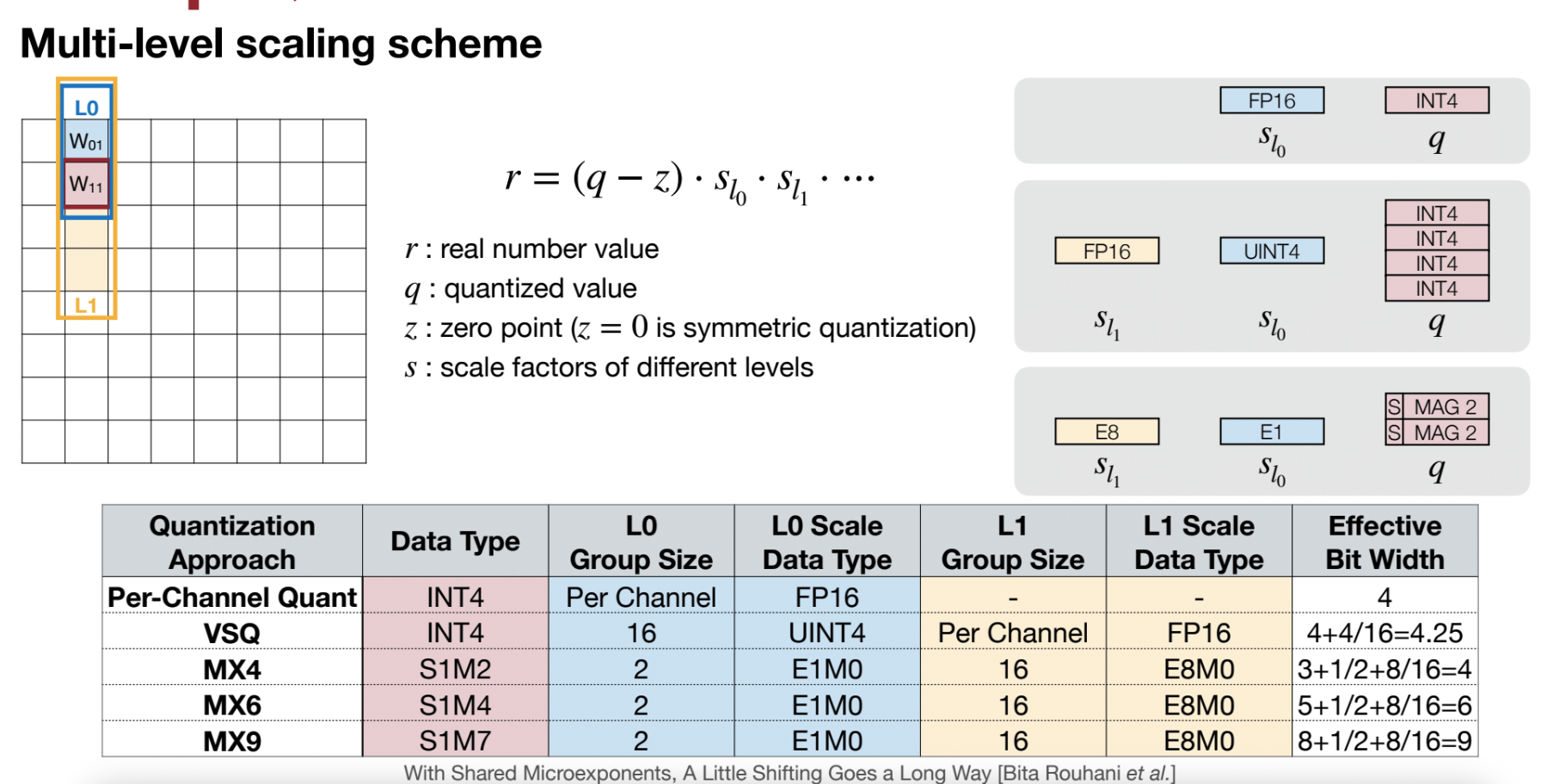
- Group quantization
- Per-vector quantization
- Shared Micro-exponent (MX) data type
Dynamic Range for Activation Quantization
If training model from scratch, we can collect statistics of the activations dynamic range using exponential moving average. $$ r_{max} = \alpha * r_{max} + (1 - \alpha) * r_{max} \ r_{min} = \alpha * r_{min} + (1 - \alpha) * r_{min} $$
where $\alpha$ is the decay factor. The observed ranges are smoothed over training steps $t$.
If we don’t have access to training data, we can use “calibration” samples on trained model.
Find activation dynamic range by minimizing “loss of information”, which is measured by KL divergence of original and quantized activation distributions.
Another optimization is minimizing mean square error (MSE) of original and quantized activation values.
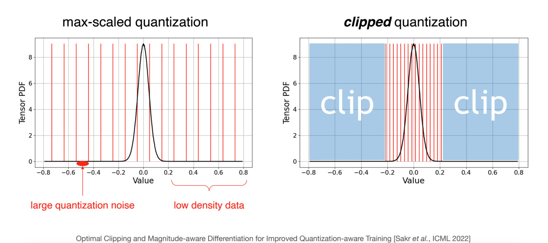
What is good quantization? Error comes from rounding the original values to the nearest precision. The intuition is that, quantization need to clip the dynamic range (instead of blindly pick min and max), so that the quantized values has good enough precision to represent the majority of original values. Avoid spreading quantized INT samples over low population ranges.
Rounding
Rounding to nearest integer is a simple and effective rounding method, but not always the optimal rounding method.
GPTQ
https://arxiv.org/abs/2210.17323
GPTQ (Generalized Post-Training Quantization) is an advanced quantization technique that uses Hessian-based optimization to minimize quantization error. Key Idea:
- Instead of simply rounding weights to the nearest quantized value (RTN - Round-To-Nearest), GPTQ uses:
- Second-order information (Hessian matrix from calibration data)
- Sequential quantization with error compensation
- Adaptive rounding that considers inter-dependencies between weights
However, comparing to AWQ, the reconstruction process of GPTQ may lead to an over-fitting issue to the calibration set and may not preserve the generalist abilities of LLMs for other modalities and domains. It also requires a reordering trick to work for some models.
Quantization Aware Training (QAT)
Add a Simulated Quantization Layer to the model, and train the model as usual.
Backpropagation pass through quantized values and is propagated to the original values.
TorchAO: https://openreview.net/attachment?id=HpqH0JakHf&name=pdf
Activation-aware Weight Quantization
https://arxiv.org/pdf/2306.00978
Quantization techniques for LLM. further push weight quantization from 8-bit to 4-bit.
LLM is highly memory-bound (weights and KV cache), especially during decoding phase with small batch size.
we need low-bit weight-only quantization (W4A8) for this setting.
It’s observed that keeping 1% of weights (Salient Weights) in full precision (W16) can recover a lot of perplexity loss.
but how to determine which 1% of weights are salient? Salient Weights should be determined by activation distribution not weight. because outliers in activation is sensitive to weight precision after multiplication. (for large activation outliers, small delta in weight precision can cause large delta in output.)
However, is it necessary to introduce mixed-precision?
Turn out by simply scaling up the salient weights channel will work. because by scaling 2x, 4x, etc, makes value more distinguishable after quantization. (i.e. 0.5 and 1 will both be 1 after quantization, after 2x scaling, 0.5 will be 0 and 1 will be 2 which is more distinguishable after quantization.)
Query-Key-Value Attention Mechanism
Project the embedding ( E ) into query, key, and value ( (Q, K, V) )
The Query-Key-Value design is analogous to a retrieval system. Let’s take YouTube search as an example:
- Query: text prompt in the search bar
- Key: the titles/descriptions of videos
- Value: the corresponding videos
Attention Formula: $$ \begin{aligned} \text{Attention}(Q, K, V) = \text{softmax}\left(\frac{QK^T}{\sqrt{d_k}}\right)V \end{aligned} $$
where $d_k$ is the dimension of the key vectors.
Questions?
- When to use which quantization technique?
- How to make trade-offs between quantization accuracy and performance? on different models?
- Any application of MX format in real model or hardware?
- what metrics to evaluate quantization accuracy? perplexity for LLM, diffusion model??
Reference
[1] EfficientML.ai, Lecture 5: Quantization, Song Han: https://www.dropbox.com/scl/fi/qc2s9opsa2mnqfithvwz1/Lec05-Quantization-I.pdf
[2] Deep Compression, Song Han, et al.: https://arxiv.org/abs/1510.00149
Advanced Quantization Schemes
https://github.com/nunchaku-tech/deepcompressor
- Post-training quantization for large language models:
- Weight-only Quantization
- Weight-Activation Quantization
- Weight-Activation and KV-Cache Quantization
- Post-training quantization for diffusion models:
- Weight-Activation Quantization